11th June 2012
Here, we provide a very informal primer to aspects of knot theory relevant to
the study of DNA topology.
 Definition:
A knot is a an embedding of a circle into R3 considered up to
continuous deformations.
Definition:
A knot is a an embedding of a circle into R3 considered up to
continuous deformations.
But what does this mean and, most importantly, why are your shoes unknotted?
Simply put, you can untie your shoes without breaking the laces. This
example, while a bit lighthearted, represents a crucial consequence of the above
definition. Let's explore this more carefully so that we can decide what
objects can and cannot be classified as knots in the mathematical sense.
A knot is an embedding, meaning our map from a circle into R3
must be injective. This immediately guarantees that a knot will never
intersect itself. An embedding is also structure-preserving
which, in this case, means that the connectivity of the circle that we started
with must be preserved. This second property begins to paint a picture of
why many objects colloquially referred to as "knots" will in fact fail to meet
the criteria of the mathematical definition: connectivity of a circle is not
preserved.
But why is this the case? If I take my shoelaces and tug on them, the
"knot" doesn't become "unknotted." If I take a piece of string and tie the
ends together, it certainly looks like I've preserved the structure of a circle
in R3. What's going on here? How far removed are these
cases from being knots in the proper mathematical sense?
They are not far removed at all! If one were to take the ends of their
shoelaces and tape them together, they would have created a mathematical knot.
How do you know? Simple: no two points on the shoelace occupy the same
point in stance, and you can't untie your shoes without breaking the tape or
cutting the string! More formally, the connectivity of the circle is now
preserved. Two points that were adjacent in the circle are now also
adjacent in the knot.
If we are to map a circle into R3, why is it useful to constrain its
topology in this fashion? The reasons are many, but here we focus on the
resulting properties of linked knots in preparation for our study of DNA.
In particular, we develop three important quantities: twist, writhe, and linking
number.
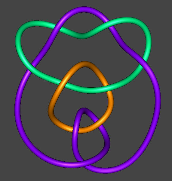
In essence, the linking number describes the number of times each curve winds
around the other. Twist describes how tightly the object wraps around
itself, while the writhe describes its orientation in space.
But all this is rather vague: let's clear the air with an example.
Consider a coiled telephone wire. Suppose we take the wire, twist it as
much as we can, and then glue the two ends of the wire together. What
happens? If we glue the two ends and then let go, the wire will bend and
contort itself in space to relieve the strain. This hints at a an
important relationship we will use repeatedly:
Linking number = Twist + Writhe
The linking number of two linked knots cannot be changed
without breaking one of the strands. Hence, once we have formed a link
between knots, the linking number is a topological invariant. We can,
however, change the twist and writhe by contorting the knots in space.
Regardless of how we do this, the twist and writhe will always be constrained by
the above equality.
As we will discuss in the future, all of this is highly applicable to DNA
topology! A closed DNA loop (such as a plasmid) consists of two linked
knots with a characteristic linking number. We will present several
methods of modelling DNA knots and loops using knot theory and differential
geometry, along with the strengths and weaknesses of each.
Images on this page were generated by KnotPlot.