25th June 2012
A primer for Legendrian Knot Theory.
We have previously discussed (1,2)
what a
"knot" is in mathematical language, how this definition differs from the
vernacular, and why it is reasonable to model certain biological phenomena using
these concepts. To explore DNA knotting and looping even further,
we introduce a special class of knots: Legendrian knots.
Before delving into what Lengendrian knots are, what sets them apart from
other knots, and why they are useful for our purposes, it is essential to first
introduce some preliminaries.
Definition: The standard contact structure
ξ0 on R3
is the z-plane field satisfying that at (x,y,z),
the normal vector is (-y,0,1) or, equivalently, the plane is spanned
by {(0,1,0), (1,0,y)}.

The idea is to assign to each point in
R3 a plane that is defined
by the coordinates of that point. As we will see, a Legendrian knot is a
knot in R3 whose tangent plane at each point is in the contact structure.
More formally,
Definition: A knot K is
Lengendrian with respect to ξ0
if at every point on K, the tangent vector to K is in ξ0.
We call two knots Lengendrian isotopic if there is an isotopy between
them which preserves the property of being Legendrian at every stage.
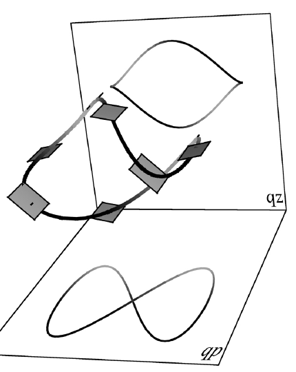 In
the figure to the right, we see an example of such a knot. Included also
are projections onto the xz- and xy-plane. We call the projection of a
Legendrian knot onto the xz-plane the front projection. In
the figure to the right, we see an example of such a knot. Included also
are projections onto the xz- and xy-plane. We call the projection of a
Legendrian knot onto the xz-plane the front projection.
In our study of DNA, we will make extensive use of the following property:
Theorem: Any diagram without vertical tangents which is smooth away from
finitely many cusps, is planar isotopic to the front projection of a Lengendrian
knot.
Hence, Lengendrian knots, while seemingly quite complicated, are very easy to
find! All we need is a diagram of a closed curve that has no vertical
tangents. Once we have done so, we can use the following property of the
front projection: If the tangent to the front projection of K at p=(x0,0,z0)
has slope m, then p is the projection of the point (x0,m,z0).
This is very useful! If we can find a diagram that has no vertical
tangents, we are allowed to say that it is an isotopy of a front projection.
Once we have our front projection, we can entirely reconstruct what the knot
looks like in R3.
Next time, we will look at how these properties can be used to illuminate
certain phenomena in genetics and medical imaging.
The images on this page are from
Grin: Publish and Find Knowledge and
What is... a
Lengendrian Knot? by Joshua M. Sabloff, published in Notices of the
AMS.
|